Playing with Fire Part 2: Using Satellite images and Cellular Automata to predict Wildfire Spread
A couple of weeks ago, I put myself to the test and build a wildfire simulation that can actually describe a real fire. This is the second part of my series on wildfires with remote sensing. I will continue with the analysis of the massive wildfire in Tasmania, Australia. In the first part, I collected the satellite images of the fire and calculated the area of the fire. Now, I will show you how to build a model that simulates how the fire spreads using the NDVI, elevation and wind.
Cellular Automaton for Modelling Wildfires 🔥
We will be using cellular automaton (CA) model, which is a semi-empirical method. That basically means that we develop a model with parameters that have to be calibrated by the actual data from part 1. If our model captures all important effects of the fire spread, then it will be able to reproduce the fire scare of the wildfire.
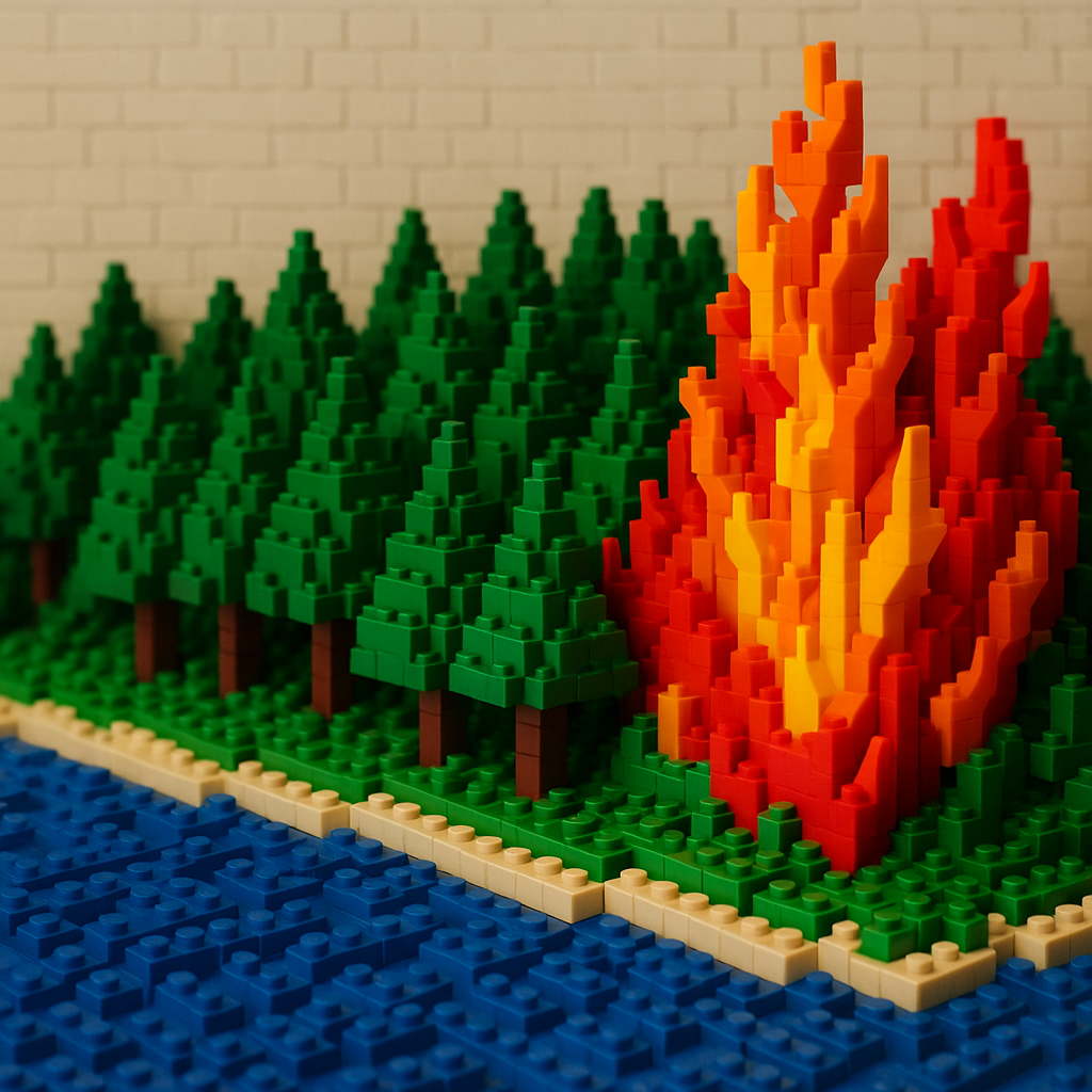
Cellular Automata are conceptually rather simple. We divide the landscape into a grid of square cells. Each cell can be in one of four states:
- Flammable (e.g., green vegetation)
- Burning
- Burnt
- Nonflammable (e.g., water bodies or bare ground)
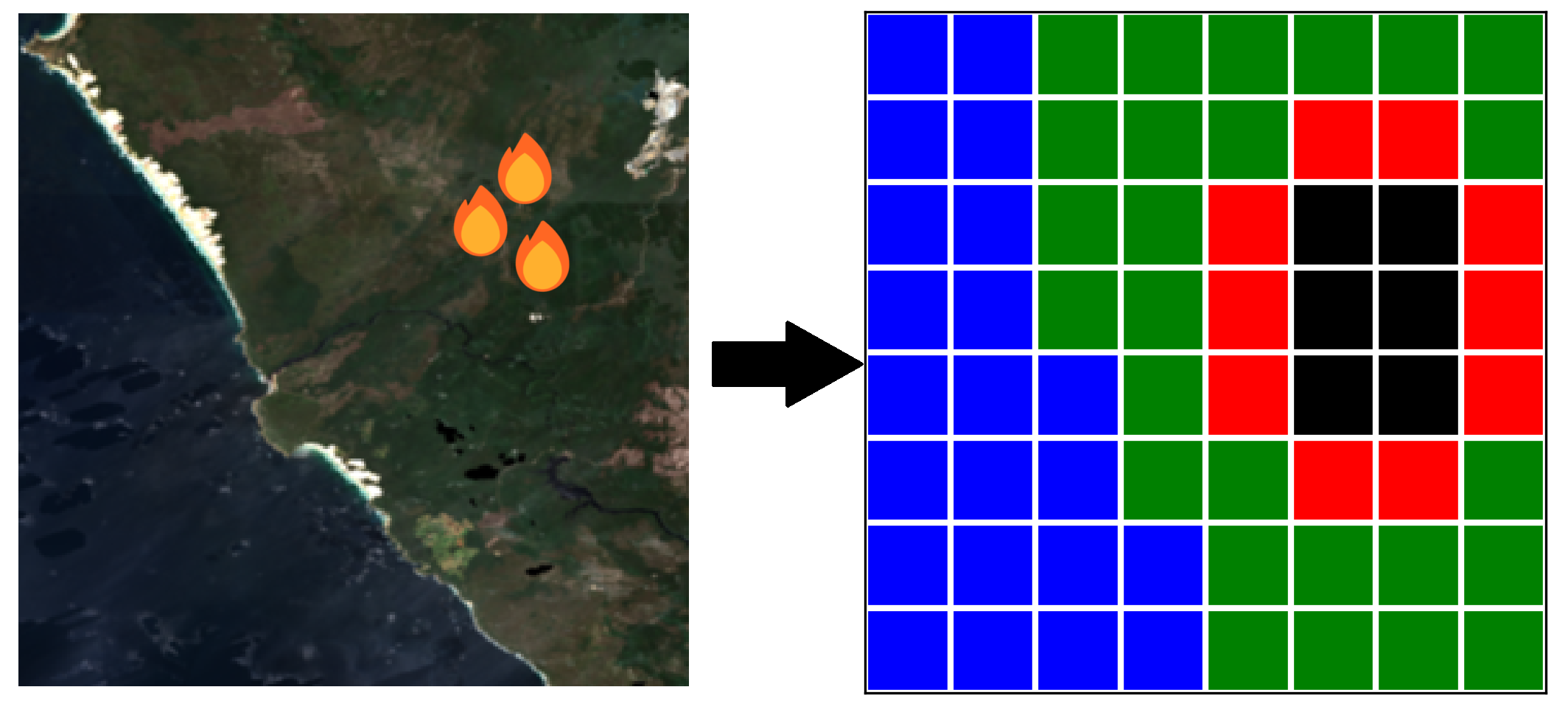
The fire propagates through transitions between these states, based on local conditions and neighbouring cells. A simple illustration is provided below — in reality, the spatial resolution is much finer than depicted here.
Rules of Fire Spread 🌲➡️🔥
Next, we define the rules of how these cells change in time.
- Burning cells (red) turn into burnt cells (black) after 1 time step
- Nonflammable cells (blue) cannot ignite, thus, they remain unchanged
- Burnt cells remain burnt cells
- Flammable cells (green) that are adjacent to burning cells have a chance to ignite given by the probability $p_\text{burn}$.
While the rules are quite simple, the tricky part is to define a realistic burn probability $p_\text{burn}$ that reflects the actual spread of the fire. I decided on using 3 effects:
- Vegetation density, quantified using NDVI
- Topographic slope, derived from a digital elevation model
- Wind direction and strength, estimated from meteorological data
Burn Probability 🎲
To model how likely a fire is to spread from one cell to another, we define the ignition probability as:
\[p_\text{burn} = p_0 \cdot f_\text{NDVI} \cdot f_\text{slope} \cdot f_\text{wind},\]Where:
- $p_0$ is a base ignition probability,
- $f_\text{NDVI}$ , $f_\text{slope}$ , and $f_\text{wind}$ are multiplicative factors for vegetation, topography, and wind conditions, respectively.
NDVI modifier For the vegetation, I divided the flammable cells into normal and densely vegetated cells, each having its multiplicative factor, i.e., $f_\text{NDVI,low}$ and $f_\text{NDVI,dense}$.
Slope modifier The slope compares the altitude of the flammable cell to the burning cell and then calculates the factor in the following way
\[f_\text{slope} = e^{c_\text{slope} \cdot (\text{elevation flammable cell - elevation burning cell})}.\]Here, upward slopes promote fire spread, since fires tend to move more readily uphill due to convective heat transfer. The parameter $c_\text{slope}$ controls how strong this topographic effect is.
Wind modifier The wind factor looks similar: \(f_\text{wind} = e^{c_\text{wind} \cdot (\text{wind speed})},\) where again $c_\text{wind}$ controls how strong this effect is. For the wind speed, we only consider the component of the wind in the direction of the fire spread. If wind is blowing from the burning cell towards the flammable cell, the burn probability is increased, if the wind is blowing the other way, the probability is reduced.
Finding the Optimal Parameters 🎯
Now that we have set up the “physics” of how the fire is spreading, we need to determine suitable values for the parameters. Let’s recap the parameters involved:
- $p_0$ : the base ignition probability
- $f_\text{NDVI,low}$ , $f_\text{NDVI,dense}$ : modifiers for vegetation density.
- $c_\text{wind}$ , $c_\text{slope}$ : sensitivity coefficients for wind and slope effects.
Now, to evaluate the results of our simulation, we compare the predicted burn pattern against observed fire data derived from satellite imagery. The standard approach is to use a confusion matrix:
| Burned in fire data (ground truth) | Unburned in fire data | |
|---|---|---|
| Burned in simulation | True Positive (TP) | False Positive (FP) |
| Unburned in simulation | False Negative (FN) | True Negative (TN) |
- True Positives (TP): Pixels burned both in the simulation and the observed satellite data
- False Positives (FP): Pixels burned in the simulation but not in the satellite data
- False Negatives (FN): Pixels that burned in the satellite data but were missed by the simulation
- True Negatives (TN): Pixels that correctly remained unburned in both cases
We can then calculate the F1 score to evaluate the accuracy of our simulation:
\[F1 = \frac{2 \cdot TP}{2 \cdot TP + FP + FN}\]- The perfect score is 1.
- The more incorrect predictions we make (either FP or FN), the lower the score.
An F1 score of 1 indicates a perfect match between simulation and observation. The goal is to adjust the model parameters to maximise the F1 score, thereby ensuring that the simulation closely replicates the spatial footprint of the real fire.
During my PhD, I worked extensively on building optimisation routines, so I am excited for this step because I have been wanting to try the Python package ‘Optuna’ for quite a while. It uses Bayesian Optimisation to efficiently explore the parameter space. This approach intelligently balances exploration and exploitation to find the parameter combination that best explains the fire dynamics.
The Result 📊
An unexpected insight from the best-fit parameters was the role of vegetation density. The model suggested that fire is less likely to spread through dense vegetation compared to more sparsely vegetated areas. Initially, this seemed counterintuitive — one might assume that more vegetation provides more fuel and therefore increases flammability. However, NDVI doesn’t directly measure dry biomass. A high NDVI indicates healthy, water-rich vegetation, which is actually more resistant to burning. In contrast, lower NDVI values can signal stressed or dry vegetation, which is more prone to ignition and combustion.
To evaluate the performance visually, the image below compares the simulated burn area to the observed fire scar extracted from satellite imagery.
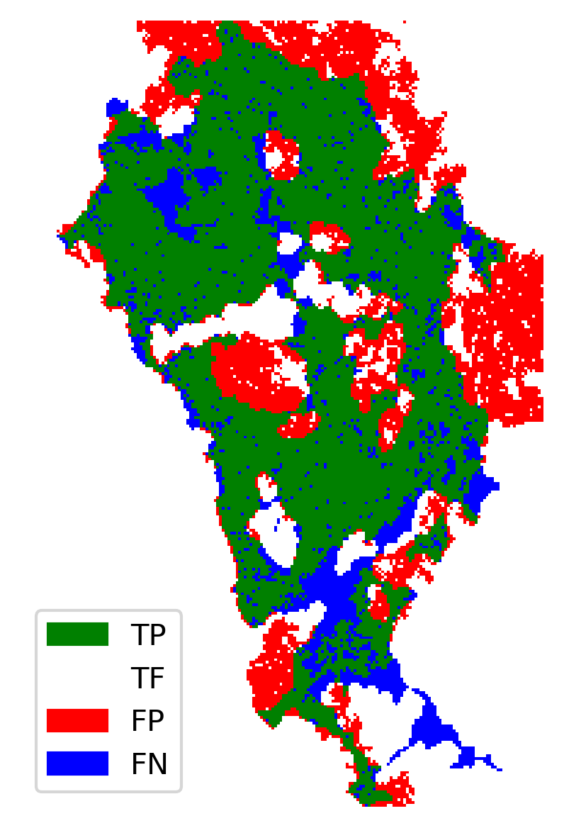
The map uses a colour-coded scheme to highlight agreement and discrepancy:
- ✅ Green — True Positives: correctly predicted burned areas.
- ❌ Red — False Positives: burned in simulation but not in the satellite data
- 🔵 Blue — False Negatives: burned in satellite data but missed in the simulation.
- ⚪ White — True Negatives: unburned in both simulation and satellite observations
Overall, the simulation captures several fire fronts accurately. In many locations, the fire halted in the simulation, where it also stopped in reality. However, there are also clear mismatches — which is expected given the simplifications in the model. For instance, the real event involved multiple ignition points, and we excluded variables such as rainfall, humidity, and ambient temperature.
I would call this a success. With just three environmental factors and a relatively simple rule-based model, we were able to reproduce a realistic fire spread pattern.
How to Improve the Model 🛠️
While the results were quite good, there are a million ways to improve on this simple model. First would be to include more/better effects into the model. Here are several factors that could be included
- Humidity
- Temperature
- Precipitation
- Vegetation moisture stress
- Vegetation type
In the current model, fires tend to extinguish when encountering unfavourable wind conditions and high NDVI (dense and likely moist vegetation). While this captures some major controls, the absence of explicit moisture and fuel-type information likely explains several overpredicted burn areas — locations that burned consistently in the simulation but not in reality. This suggests that a missing suppressive factor (e.g., recent rainfall, soil moisture, or fuel discontinuity) played a role.
Another key area for improvement is the fire spread rate. At present, the model assumes a uniform rate of 1 cell (250 m) per hour, which is too fast. Thus, the location of the fire front does not match the time-sensitive wind data. A more data-driven approach would involve estimating the real-world spread velocity using VIIRS active fire detections (the data and an ansatz are available in the Jupyter notebook). By measuring the temporal and spatial growth of the fire scar from the ignition point to the observed perimeter, we could better calibrate the spread dynamics.
Finally, the burn duration per cell is likely too short. In the current setup, a burning cell becomes burnt after a single time step. This limits the potential for accumulation and reinforcement of nearby ignition. A more realistic model would allow a cell to burn for multiple time steps, with a lower probability of ignition at each step. This adjustment would create slower fire fronts in the absence of wind, while enabling faster propagation when aligned with wind direction, mimicking real-world fire behaviour more closely.
Recap 💭
The long-term goal of such a simulation is to predict wildfire spread in near real-time or to identify high-risk areas before ignition. Achieving that level of robustness requires training the model on many different fire events. This, in turn, demands a curated catalogue of wildfires — including ignition dates, burn perimeters, durations, and satellite observations.
The pipeline developed in the first part of this project offers a path forward. By automating the extraction of key fire attributes (e.g., ignition date and burnt area masks), we can begin building such a dataset systematically.
At the moment, our model is good at predicting this particular fire, but it will very likely perform much worse on other fires. To get a model that can accurately predict the spread of any fire, we need to train it on many fires. We can follow the usual machine learning methodology.:
- Split A large dataset into a train and test dataset.
- Train the model on many fires.
- Evaluate performance on unseen fires to measure generalisation.
- Validate robustness across regions, seasons and vegetation types.
If successful, the model could be used to:
- Assess how climate change affects wildfire behaviour (e.g., under hotter, drier conditions).
- Predict fire paths for use in preventative burns or emergency response planning.
- Evaluate land management strategies by simulating alternative scenarios.
Overall, I am really happy with the result of this little project. The progress was really slow in the early stages (gathering data and getting used to the different APIs). Once the data was prepared, the development of the simulation and evaluation framework progressed smoothly without any major hiccups.