Playing with Fire Part 1: Using Remote Sensing to calculate Wildfire damages
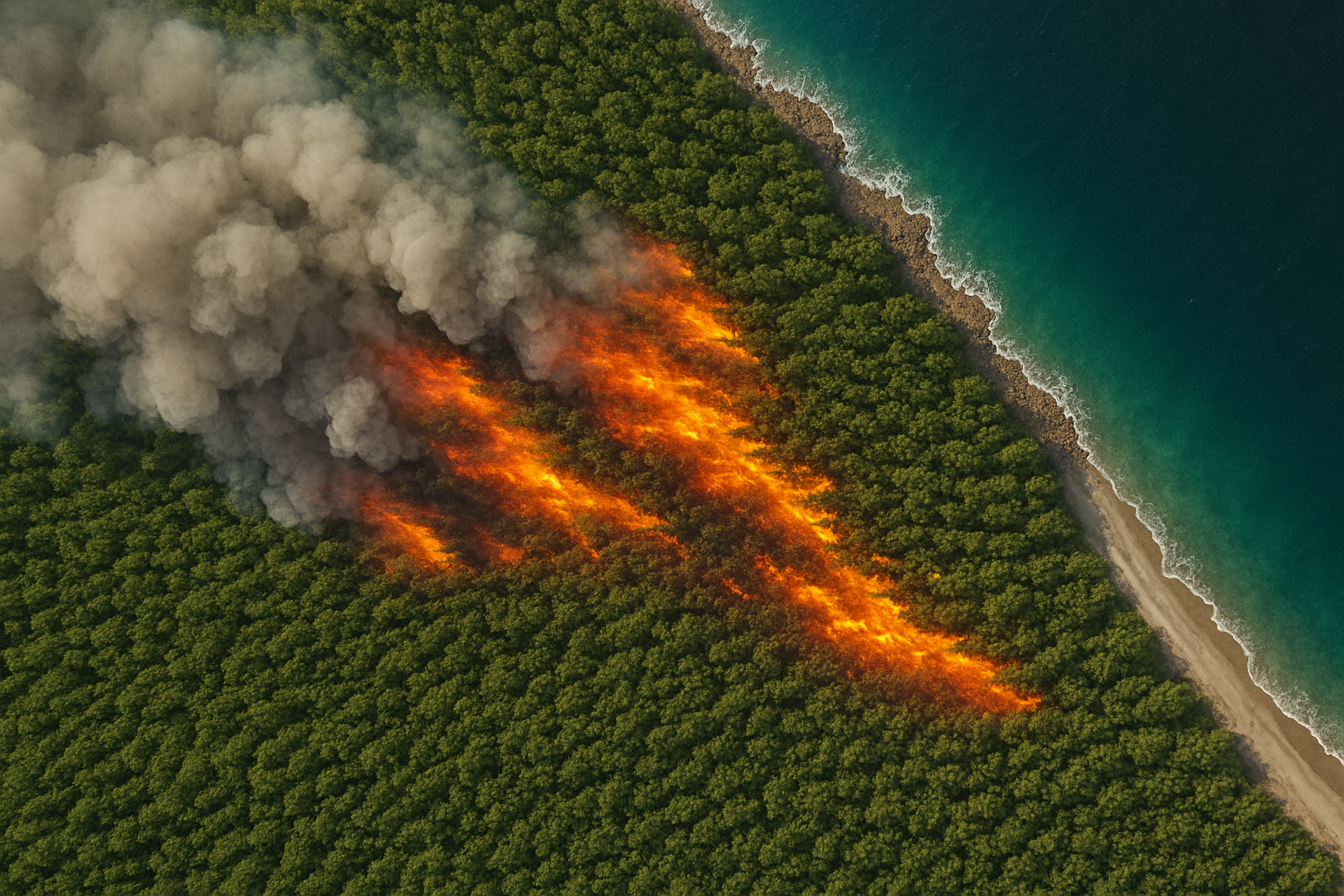
Wildfires are becoming increasingly frequent and severe — not just in traditionally fire-prone regions, but even in places like my home country Germany. Understanding how wildfires behave is crucial for mitigation and response planning. In the first part of this series, I use remote sensing data from the Sentinel-2 satellite to estimate the area affected by a wildfire. In the next blog post, I will use this data to build a “realistic” simulation that models how the fire might have spread across the landscape.
Find the code on GitHub and the Jupyter Notebook of the analysis.
Fire Selection 🔥
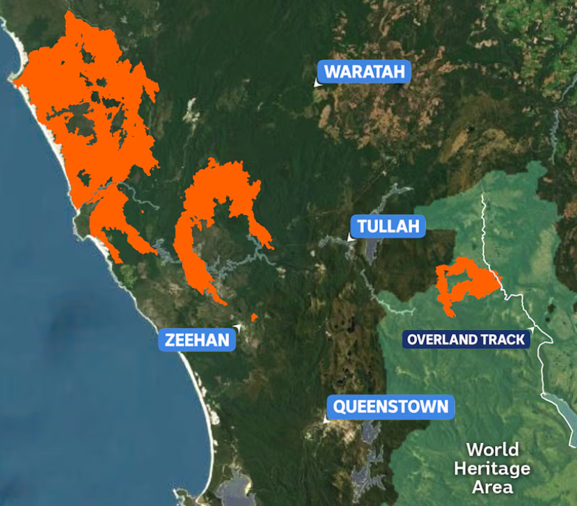
For this project, I chose one of the largest wildfires of 2025 (so far): a February bushfire in remote western Tasmania, Australia, which affected nearly 100,000 hectares. I picked this fire because it was covered in a press release that included a map of the burned area, along with key metadata such as the ignition date and total area impacted.
The ignition date was reported as February 3rd, 2025, which I confirmed using the VIIRS fire detection data from the Suomi NPP satellite, which also gave me the ignition point occurred: 145.05249° longitude and -41.57241° latitude.
Several platforms host satellite data, many of which offer APIs to download data programmatically. I initially explored NASA’s Earthdata catalog, but ultimately settled on Google Earth Engine, as I was keen to use imagery from ESA’s Sentinel-2 satellite that is available on Google Earth Engine.
Sentinel-2 data is great for this type of analysis: it has a high revisit frequency over Australia and provides data in 12 spectral bands at a resolution of 10–50 meters, which is excellent for burn scar mapping.
Data Collection 📦
So now, I “just” had to download the data.
Just.
During my PhD, I worked extensively with another ESA satellite — the Planck Surveyor — which looked away from Earth to measure cosmic radiation. So, this blog post will cover the struggles I faced when working with Earth-facing satellites
Well, the first struggle was figuring out what data is out there, what data I need for this project and how to retrieve the data from a Python script. Around 90% of the project was spent on this part, as every image I downloaded seemed to arrive in a different file format, which I had not heard of until then. Learning new things usually goes through 3 stages, which roughly go like this:
- “Why are they using
.hdffiles and not just.txtfiles?” - “Oh…
.hdffiles are actually quite handy. Makes sense.” - “WHY is this not saved as
.hdf?!”
Eventually, I overcame the initial struggles and managed to automate the download process via Google Earth Engine, apply cloud masks, and set up the whole data collection pipeline. Installing heaps of libraries such as GDAL, xarray, rasterio, etc. The rest of the project was a breeze once all the functions were in place to download cleaned satellite images quickly.
Remote Sensing and Spectral Indices 🛰️
Now that I have the satellite data ready, we can dive into the core of the project: using remote sensing to detect and quantify fire damage. Here is a quick summary of what remote sensing is.
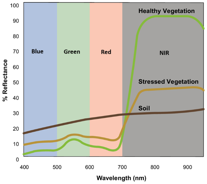
Remote sensing involves gathering information about the Earth’s surface from a distance, typically using satellites equipped with sensors that record reflected sunlight across various wavelengths. Multispectral satellites like Sentinel-2 record data in multiple spectral bands, including visible light (red, green, blue) and invisible wavelengths like near-infrared (NIR) and shortwave infrared (SWIR). This opens up two powerful approaches for analysing the land surface:
- True-color imagery, where red, green, and blue bands are combined to form an image similar to what we’d see with our own eyes.
- Spectral indices, which calculate the contrast between different wavelengths to reveal patterns invisible to the naked eye.
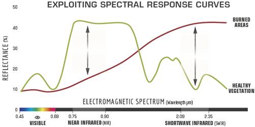
One popular example is the Normalised Difference Vegetation Index (NDVI). It takes advantage of the fact that healthy vegetation reflects much more NIR radiation than red light. By comparing these two bands, we can map the density and health of vegetation. This is shown on the left. Similarly, to detect areas affected by fire, we use the Normalised Burn Ratio (NBR). This index compares NIR and SWIR reflectance. Burned vegetation reflects more SWIR and less NIR, making the NBR an effective tool for identifying burn scars. This is shown on the right below.
Calculating Burnt Area with dNBR 🧮
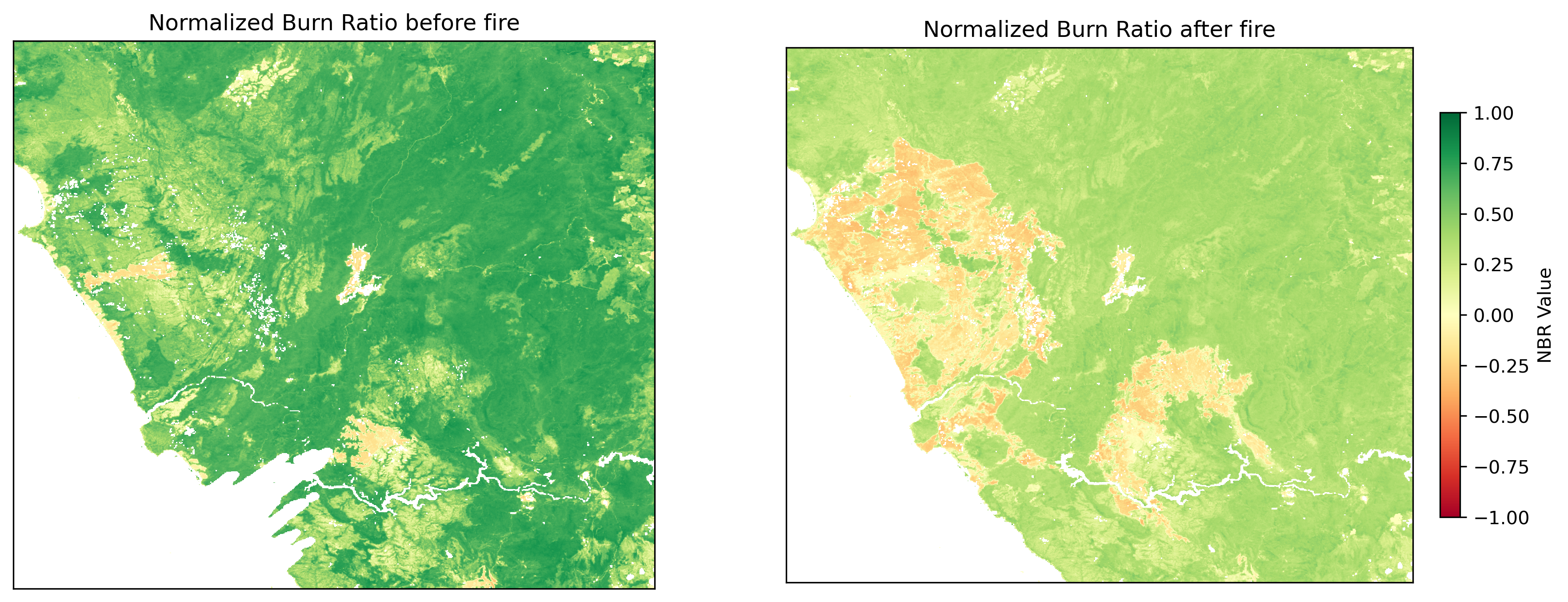
Now, we collect satellite data from before the fire and after the fire. The next step is to calculate the Normalised Burn Ratio (NBR) before and after the fire. By comparing these two NBR images, we can pinpoint the areas affected by the fire.
In the first image below, you can see the NBR calculated just before the fire (left) and after the fire (right). You’ll notice some white patches — those are clouds. Kind of ironic: in cosmology, we launch satellites to get above the clouds and avoid atmospheric interference, but in remote sensing, clouds are one of our main obstacles. To reduce their impact, we can combine multiple satellite captures taken over different days to stitch together a cloud-free view. Here, we have to strike a balance between getting clean pictures and getting recent pictures.
I also excluded pixels classified as water. That’s because water can have wildly varying NBR values and is easily mistaken for burned vegetation. Fortunately, Sentinel-2 provides a Scene Classification Layer (SCL), which automatically tags each pixel as land, water, cloud, shadow, etc. We used that to clean the data before proceeding.
To better highlight the fire damage, we calculate the difference in NBR (dNBR) between the two images. In the image below, brighter areas (white) indicate no major change, while darker browns to reds show where the fire caused significant vegetation loss.
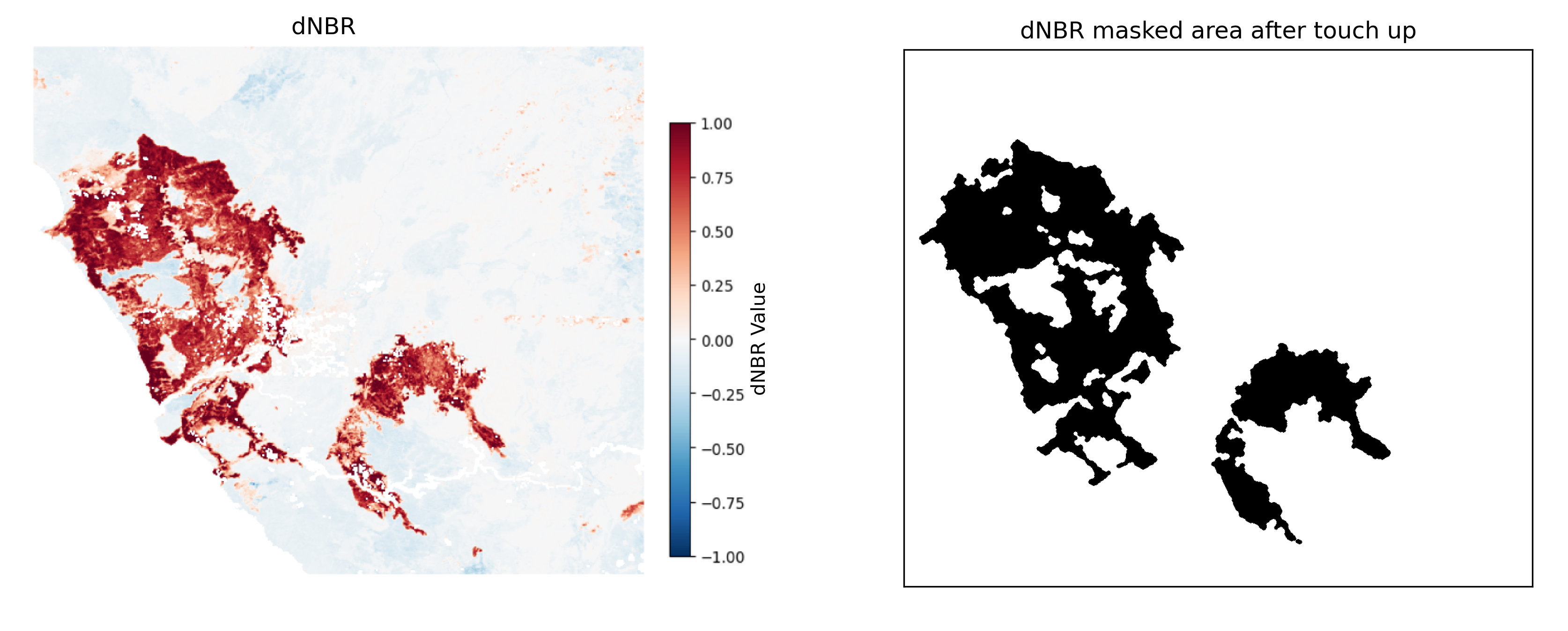
The final step is to classify pixels as “burned” based on a dNBR threshold. I went with a threshold of 0.15, though even thresholds as high as 0.3 gave visually similar results. Then I cleaned the final fire area by
- Removing tiny isolated patches
- Filling in small internal holes
- Smoothing the boundaries
Results 📊
Using the cleaned-up dNBR map, we can now estimate the total burnt area. By counting the burned pixels and multiplying by the pixel with their resolution, we get that roughly 80.000 ha of burnt land, which aligns well with what was reported in the news article, excluding a small fire area on the right that I didn’t include in my mapping.
And this is how remote sensing can be used to calculated the area of a wildfire. Quite amazing how we used two radiations (near infrared and shortwave infrared) that are invisible to the naked eye and were able to clearly map the burnt area.
Keep your eyes peeled for part 2, where I will build a simulation that can model the spread of the fire.