Orbit to Oak: Mapping Biomass from Space
We all know that forests store carbon, but can we estimate the amount without local measurements? And if yes, how accurate is the estimate?
In this project, I used GEDI LiDAR data as “ground truth” for aboveground biomass and paired it with optical and radar satellite data to predict biomass across a German forest.
The concept is simple: we give the machine learning algorithm examples of where biomass is high or low (from GEDI) and the corresponding “satellite fingerprints” from multiple data sources. Once trained, the model can scan the whole landscape and estimate biomass everywhere.
Data processing and resampling were done in Google Earth Engine, and the prediction model was built with XGBoost.
🌍 Ground Truth
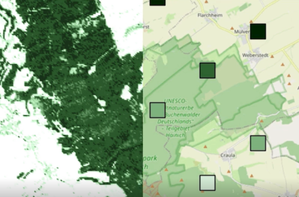
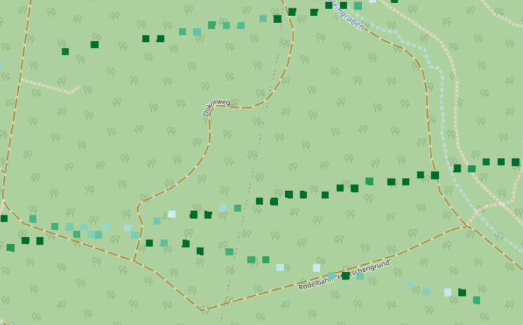
GEDI (Global Ecosystem Dynamics Investigation) is a LiDAR laser mounted on the International Space Station. It measures the height and structure of forest canopies, allowing us to estimate aboveground biomass density. Each measurement covers a footprint of roughly 25 m × 25 m, but these points are sparse, only covering fractions of a forest as shown in the image below. The squares are showing the GEDI footprint with green being high biomass density and white low.
🛰️ Predictors
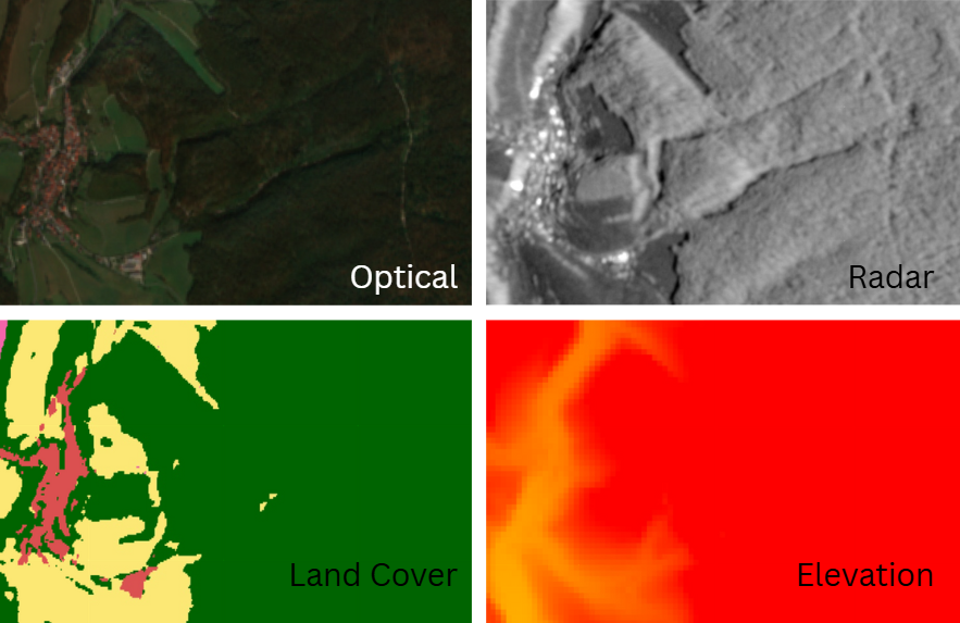
To fill in the gaps between GEDI shots, we can use other satellite data as predictors:
- Optical & multispectral (Sentinel-2) for vegetation health and structure
- SAR (Sentinel-1) for texture
- Elevation and land cover for context
combining these with the GEDI biomass estimates, we can train a model to map biomass continuously over the whole region.
The idea is simple: each GEDI footprint comes with both a biomass measurement and its corresponding values from all these predictor datasets. The model looks for patterns, for example, high NDVI and dense SAR returns often mean high biomass, while bare soil or urban areas have low biomass.
By learning these relationships from known points, the model can then predict biomass for every pixel in the area of interest, even where no GEDI measurement exists. This turns the sparse GEDI points into a continuous biomass map.
📊 Regression
I used XGBoost (a powerful regression tool) to link GEDI biomass measurements with the predictor layers. GEDI has a baseline uncertainty of about ±7 Mg/ha, which can make low-density areas tricky to model. My final model achieved an RMSE of ~50 Mg/ha (≈40% uncertainty).
Not perfect — but given the noise in GEDI, not bad either. Slightly better than what I found in tutorials. Below, we can see which features were the most important ones for the prediction.
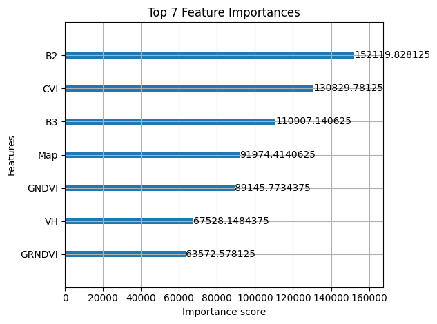
Above, we can see which features helped the most for predicting the biomass. B2 is the blue colour band and B3 the red colour band of Sentinel 2. CVI is the Chlorophyll Vegetation Index. There are a few more vegetation indices (GNVDI & GRNDVI), as well as the radar information (VH) and the land cover (Map). The importance of features strongly varies depending on the type of forest.
🌲 Results
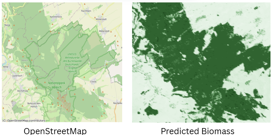
Visually, the predictions made sense: dense forests lit up with high biomass, open areas stayed low. Still, I was hoping for 10–20% uncertainty, but diverse landcover types probably made this harder.
Other studies using larger, more homogeneous forests report RMSEs around 30–40 Mg/ha, and in cases with actual ground measurements, even ~20 Mg/ha.
From biomass, we can estimate stored carbon. A rough estimate is that around 50% of the aboveground biomass is carbon, the forest in my study area has an average aboveground biomass density of 135 kilotonnes per hectar, leading to 3 megatonnes of carbon.
💭 Final Thoughts
If I had actual field biomass data, I’d love to see how it stacks up against GEDI. The GEDI dataset was messy, and simpler models often worked better to avoid overfitting to noise.
Another interesting application would be to see how the aboveground mass of the forest is changing over time. Forests are often called carbon sinks, meaning that they absorb carbon. This would be true if the biomass of the forest is increasing over time, which is true for healthy forests.
A side note: the Google Earth Engine Python API is slow for large downloads to disk — even a few MB took ages. Doing everything in the JavaScript Code Editor is faster, but its regression options are limited.